This page goes through the steps of the discrete calculation of the payoff to 'var' vs. any fix(x). It gives an inexact solution that, if the cost values are close to each other, approximates the exact solution we saw earlier (given by calculus). This page is especially useful for those who have not had calculus since it should help them to understand how costs, benefits, and payoffs are calculated. It should also help anyone to see how this site's war of attrition computer simulation finds solutions and why the calculus solution is more exact than the one obtained by a computer. Accompanying this sheet is an Excel worksheet that will allow you to see the discrete calculation in detail and see the effects of changing cost intervals and V on benefit, cost, and payoff plots. You need a recent version of Microsoft's Excel ('97. '98 or later) to use this sheet. |
This page gives you an idea of how a computer calculates the fitness of our mixed strategist 'var'. If you are not familiar with calculus, it is an excellent way to understand the effect of calculus solutions. Every operation used here will be familiar to you if you have completed high school algebra. Besides learning how a discrete solution is reached, you will also have a chance to see how computationally intensive this type of solution is (one of the reasons that calculus was invented was to avoid this type of solution). You'll also see that the discrete calculation is inexact -- it becomes more exact only as more and more computations are made but it never reaches the degree of precision that is obtained through calculus.
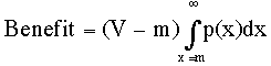
As always, the expected lifetime payoff to 'var' against fix(x=m) is the difference between the net benefit to 'var' when it wins and the costs when it loses. What follows are the means of calculating each of these:
Net Benefit in Wins: Recall that for each value of m that a fix(x) strategist plays, there is a certain chance that 'var' will win and a unique V-m for that value. 'Var' wins whenever fix(x=m) quits first. Recall that our calculus formulation for net benefit in wins is:
eq. 14a:
We said earlier that the chance that 'var' will not have quit as of a certain cost x=m is called Q(m). Therefore:
eq. dc1: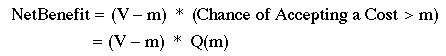
and if we integrate the probability density function, p(x), for all winning costs (i.e., all costs between m and infinity) we get Q(m):
eq. dc2: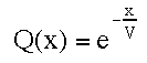
The integration that gave us Q(m) gives a result that is functionally nothing more than adding the probabilities of 'var' playing all costs that are greater than m. Since the result of the integration is a simple equation that a computer can easily solve (since computers have built-in natural log functions -- although they calculate logs in way that no sensible human would but that plays to their strength -- doing repeated calculations very quickly) then, we will use this equation (# dc2) anytime we need Q(m).
So, our equation for net benefit is:
eq. 14b:![]()
which is the same equation we used earlier for calculation of net benefit.
When computers are used to solve problems involving a range of values of the independent variable (x), they do so by calculating for relatively large (discrete) steps of x. Here a short list of solutions to eq. 14b (net benefit) where x=m increments by 0.01 units (we'll call this value "delta x"):
x=m |
Q(m) |
(V-m) |
Q(m)*(V-m) |
0 |
1.0000 |
1.000 |
1.0000 |
0.0100 |
0.9900 |
0.9900 |
0.9801 |
0.0200 |
0.9802 |
0.9800 |
0.9606 |
0.0300 |
0.9704 |
0.9700 |
0.9413 |
0.0400 |
0.9608 |
0.9600 |
0.9224 |
0.0500 |
0.9512 |
0.9500 |
0.9037 |
Now nothing that we have done so far is any different then when we solved for net benefit earlier. But the next section will be quit different.
Costs in Losses: Recall that losses that 'var' incurs to a given fix(x=m) happen any time that 'var' quits before m. Now the problem is that 'var' can quit at any cost before m. So, for all values of cost below m there is a unique chance that 'var' will quit at each of these costs. Now since we want to know the costs that 'var' will quit before m, the lifetime cost 'var' pays in many contests with any fix(x=m) is the sum of the product of each losing cost and the probability of actually losing. Previously, we wrote this as:
eq. 16a: 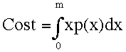
which says that for every cost between 0 and m(i.e., for every cost where 'var' loses to fix(x=m)), we need to multiply the each losing cost x times the chance of losing at that particular cost and then add this to all other losing costs.
We can express this in a nearly equivalent manner as:
eq. dc3: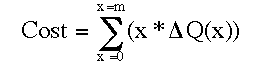
This is a discrete formulation of eq. 16b. Let's see what it says to do. Once again, for each losing cost that 'var' plays (between x=0 and x=m), multiply the cost times something called 'delta Q(m)".
eq. dc4:![]()
Now for an important point. Unlike with eq. 16a, in eq. dc3 we are calculating all the quits that occur in what is potentially a large cost interval (m1 to m2) and multiplying this number by a single cost, the cost x which equals either m1 or m2. This is bound to introduce some error in our calculations since clearly cost x did not apply to all quitting chances between m1 and m2. So the discrete solution (unlike the calculus solution) is always an approximation. But, we'll see that these errors can be made to be relatively small, if the increment m1 and m2 ("delta m") is also small. (Doing this makes the solution more like a calculus solution).
This is probably all very confusing. It should make more sense if you follow through the calculations below.
OK, now we have a means to calculate the expected net benefits and costs that var would experience against any fix(x=m). To find the payoff to var in these contests then, we simply subtract costs from benefits:
eq. dc5: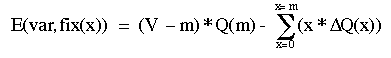
Here is the calculation of payoffs for m = 0 to 0.05 in steps of 0.01. We use the values of benefits and costs that were calculated above. For comparison, the payoff calculated from the exact (calculus) solution is given in the green column; the difference between the discrete and exact calculations is given in the purple column:
Cost that Fix(x = m) Opponent is Prepared to Pay |
Expected Lifetime Net Benefit to 'var' for wins against fix(x=m) Q(m)*(V-m) |
Expected Lifetime Cost to 'var' in contests that it loses to fix(x=m) |
E(var, fix(x=m)) Calculated Discretely for 0.01x steps of cost |
Exact Value (from eq. #19b) |
Discrepancy (discrete - exact) |
0 |
1.0000 |
0 |
1.0000 |
(1.0000) |
0 |
0.01 |
0.9801 |
0.0000995 |
0.9800 |
(0.9801) |
-0.0001 |
0.02 |
0.9606 |
0.000296 |
0.9603 |
(0.9604) |
-0.0001 |
0.03 |
0.9413 |
0.000589 |
0.9407 |
(0.9409) |
-0.0002 |
0.04 |
0.9224 |
0.000975 |
0.9214 |
(0.9216) |
-0.0002 |
0.05 |
0.9037 |
0.001453 |
0.9022 |
(0.9024) |
-0.0002 |
Notice that in this case, the discrepancies are small. Recall that all discrepancies are due to the fact that in the cost calculation it was assumed that on all occasions when an individual quits in a given delta m (cost interval), it paid the same cost. The reason the error is so small is that the cost interval is small -- larger cost intervals result in larger and larger errors.
If you wish to see this for yourself and if you have a recent version of Microsoft Excel (ideally the version that comes with Office '97, '98 or later), press here to get a spread sheet where you can alter the size of the cost steps or V.
Copyright © 1999 by Kenneth N. Prestwich
About Fair Use of these materials Last modified 3- 14 - 99 |