Instructions for the War of Attrition Game

The War of Attrition Simulation

Synopsis: This page explains how to use the three modules in thewar of attrition simulation. This page also suggests things to try withthe simulation and it asks a number of questions that you should be ableto answer with the help of the simulation or hypertext.

Contents:

Introduction
How to use the simulation and suggestions for things to try:
Go to the simulation
Bottom of this frame

Introduction: There are three "modules"to the war of attrition simulation:

The Q(x) Calculator
Single Game Simulation
Multiple Game Simulation

The Q(x) calculator, uses up to three different values of V toconstruct plots of the chance that a mixed ("var") strategistwill play up to some cost x. It is a good way to become familiar with theeffects of V on quitting.

The single and multi game modules are considerably more complicated.Both allow you to define the resource value (V) and the strategies usedby two contestants.

If you select single game you will see the progress of a gamedepicted by a graph of cost vs. time. When the game ends, a summary graphshowing the costs and benefits received by each contestant will appear.This game is an excellent chance for you to review you understanding bothof fixed and mixed strategies and the calculation of benefits and costsin the war of attrition.

If you select the multiple games module, the computer will playup to 5000 contests and then present a summary of the quitting times andpayoffs. If one or both of the contestants is a var strategist, itwill also draw a theoretical plot of quitting times which you can comparethis with the observed pattern. Clearly, this simulation will be most usefulafter you have gained a general understanding of the war of attrition fromreading the hypertext materials presented elsewhere at this site.

Back to the contents and top of this frame
On to the simulation

Notes Regarding Different Platforms

Notes to Windows Users: This simulation has been testedon machines running Windows95 and NT using Netscape and Internet Explorer3.x and 4.x.
If you use Netscape or Explorer 3.x for Windows, be advised thatthe colors of various windows objects (buttons menus etc.) will notbe as described -- most will be in the background color (supportfor color is poor in this release).
Please remember that Java does not work on any version of windowsprior to Windows95.

Notes to Macintosh Users: This simulation has been testedon machines running Mac OS 7.6, 8.1 and 8.5 using Netscape 4 and 4.5 andInternet Explorer 3, 4, and 4.5.
If you are using Explorer, and have Apple's MRJ installed (a featureof OS 8.1 and 8.5, it can be gotten by pressing here if using an earlierOS), I recommend that you set the MRJ as the default Java for the Browser.To do this, go to the EDIT menu item, select "Preferences"and open the "Web Browser" menu (on the left side of thePREFERENCES dialog box). Then, select "Java". In the dialogbox at the right, be sure that Java is enabled and that "AppleMRJ"is selected from the choice menu near the top. Restart Explorer andyou're ready to go. Failure to make this change will mean that manyobjects (buttons etc.) will not be colored but will simply have the screenbackground color. I have attempted to use color to help make the layoutof the various windows easier to understand.

Back to the contents and top of this frame
On to the simulation

General Navigation: Thissection tells you how to get around the program. If you are comfortablewith computers, you can probably skip it and move onto the detaileddescriptions of the modules.

On starting the program, you will see the following screen:

The buttons at the bottom will give general information (blue) aboutthe simulation or will send you on (red) to the next screen which containsa menu of the simulations:

The information button on this menu summarizes the features of each ofthe three simulations. Pressing one of the lower buttons will take you tothat particular simulation and will hide this "menu" window. Oneimportant point -- notice that when you go to this window, the start-up window will remain visible in the background.You can get back to the "Select The Version of the Simulation"(menu) window at any time by going to the start-up windowand pressing "Continue".

Detailed OperationalDescriptions and
Instructions for Each Module

The Q(x) Calculator: This is a simple calculator/graphingutility to allow you to review the effects of V on a mixed ("var")strategist. Using the setup screen depicted below enter up to three differentvalues of V and press the red "View" key:

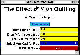
Remember our convention that all resources must have values greaterthan zero -- entry of values =< 0 in any of the textfields orentry of any non-numeric characters will generate an error warning windowlike this one:

Simply close the error window and re-enter the data.

The resulting output window (below) consists of two coordinate axes.The top graph gives the chance of playing from a cost of zero to a particularcost x. Thus, it is a plot of Q(x) vs. x. A legend tellsyou which plot goes with which value of V:

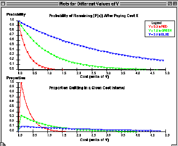
The lower graph is a bit harder to understand. It shows the relativeproportion of individuals who quit in any given cost interval. Recall thatthis is the difference between Q(x) and Q(x-1).

All of these data are referenced to the greatest number of individualsto quit on any of the three plots. For example, say that between a costof 0 and 0.05 that:

Value of V
Proportion Quitting for a Given V
0.3
0.154
1.0
0.049
3.0
0.017

(note: this first interval must always be where the greatest number (proportion)of quits occur (you should know why -- if not review the hypertext). So,the program will find that the greatest proportion to quit between cost= 0 and 0.05 occurred where V = 0.3 which is 0.154 (see table).

It will then normalize all other values against it. What this means isthat the values at all other cost intervals for all other values of Vare divided by this number.

Value of V
Proportion Quitting for a Given V
Normalized Proportion Quitting for a Given V
0.3
0.154
1.0
1.0
0.049
0.32
3.0
0.017
0.11

The advantages to doing it this way are that it emphasizes the differencein the quitting rates at different values of V.

Q(x) Calculator --Things to try and/or to think about:

Investigate the general shapes of the Q(x) curves and their relationship to the relative proportion quitting curves.
Be sure that you understand why all of the curves at the bottom start at zero, reach a maximum in the first cost interval, and then decrease. Be sure you understand how both types of curves are calculated.
Be sure that you understand why the lower values of V always have greater slopes on both graphs. Be able to explain this not just in terms of mathematical operations but more importantly, explain what this pattern means biologically and why it makes sense biologically.

Back to the contents and top of this frame
On to the simulation

The Single and Multigame Modules: How theyWork

The heart of both of these modules are computational routines for decidingwhen a contest ends and who has won.

What follows is a description of how these routines work. Reading thisdescription will not only help you understand the war of attrition but alsoit will help you understand the usefulness and limitations of these simulations.

Here goes:

The computer first looks up the strategies employed by each contestant and the present cost of the contest.
Then comes the complicated part -- determining each contestant's status (continue or quit).
- For any fix(x) strategists, it simply determines if the present cost is equal to or greater than the maximum cost the strategist will pay. If so, it declares that this particular contestant has quit.
- If the contestant is a mixed 'var' strategist
  - the routine generates a pseudorandom number
  - it compares it with the probability that a 'var' strategist will quit in any cost interval. Here's how it works:
  - Remember that for a given cost interval delta x, the probability of quitting is a constant equal to exp(- delta x / V).
  - If the pseudorandom number is less than or equal to (<=) the probability of quitting per delta x, the contestant is defined as quitting.
  - Otherwise, it is defined as continuing.
  - Notice that this calculation ensures a constant chance of quitting per delta x that is equal to exp(- delta x / V)
  - That is because a pseudorandom number generator produces numbers between 0 and 1.00 with equal probability.
  - Thus, the chance of generating a number less than or equal to exp(- delta x / V) is equal to exp(- delta x / V)
Once the program knows each contestant's status (continue or quit), it simply looks to see if the contest is over (one or both contestants have quit).
- If the contest is over, it decides who has won (i.e., not yet quit) or if there is a tie (both quit).
- On the other hand, if the contest continues the program increments the cost by delta x and performs the calculations again for the new cost.

Now that you understand how the program works, a few important pointsthat affect its behavior can be made.

Cost is not incremented continuously and observations as to who is still playing are not made instantaneously. The program makes calculations at discrete intervals only
Thus, notice that if a fix(x) strategist quits at some cost between x and x + delta (x), the program will not know exactly when the quit occurred! For instance, if delta x = 0.05 and one individual quits at 0.06 and the other at 0.09 the program will believe that a tie has occurred! Why is that? At a cost of x = 0.05, the program checks and sees that both of these fix(x) strategists are still playing (since the present x is less than both of their maximum costs which are 0.06 and 0.09). The program now increments the cost by 0.05 to x = 0.10. It then determines both contestants have quit and declares a tie!
So, the size of the cost increment also equals the limits of resolution for the simulation

To avoid problems with resolution:

When setting fix(x) strategies, always define x in as a whole number multiple of delta x.
Thus, if delta x is 0.05, then use values of fix(x) such as 0.05, 0.10, 0.15 etc. -- don't use values like 0.09 or 0.088. Likewise, if delta x is 0.01, use costs to 0.01, not something less (e.g., 0.001).

Back to the contents and top of this frame
On to the simulation

The Single and MultigameModules -- Setup Features in Common to Both Modules

From the general menu window, select either the "Introduction-- Single Game" (green) button or the "Advanced:Many Games" (gold) button. These will bring up slightlydifferent versions of the same setup window and will cause the menu screento disappear.

Reminder -- to get back to the menu screen, findthe start-up window and press the button labeled"Continue".

Here is the single game version of the setup window:

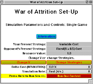
After the title and the ubiquitous "Information" button (whichreiterates much of the material about to be covered in this hypertext),the window can be thought of as having three sections:

a section common to both single and multigame simulations. It displays the present resource value V, the strategies of the two contestants and a choice menu labeled "Delta Cost (RESOLUTION)". More about this in a moment.
beneath this there will be one or two additional choice items whose identity depends on whether or not single of multiple games are being setup. For instance, in the single game setup (see above) there is a choice for "Simulation Rate" while in the multigame version the choices are "Number of Games Played" and "Output Plot's Maximum Cost".
lastly, there is a button labeled either "Run One Contest" or "Run Multiple Contests" that starts the simulation.

Changing Resource and Strategy Values

Below the display of present V and strategy valuesare two yellow and red buttons. Pressing these will bring up a dialog boxfor changing either V or strategies.

Changing V: As we have learned, the netpayoff to a contest winner is partially determined by V as is the quittingrate for the mixed 'var' strategy. Thus, there will be situations whereyou want to change these values. Pressing the yellow button labeled "ChangeV" will bring up the following dialog box:

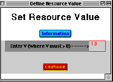
To change V, simply highlight the presently displayed value by eitherdouble clicking the cell or by clicking dragging across the part of thevalue you wish to change. Alternately (of course) you can simply click inthe cell, delete and then re-enter data. When you are satisfied with theresult, press the continue button and you will return to the "Set-UpMenu" where the new value of V will be displayed. You can changethese values as often as you wish.

Changing the Contestant's Strategies:Starting from the Set-Up Menu, pressing the buttonlabeled "Change Strategies" will take you to the following dialogbox:

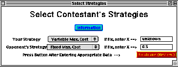
On the left are choice menus for the two contestants, arbitrarilylabeled "your strategy" and "opponent's strategy".Both give you the choice between selecting a fixed and variable cost strategy.

If you select fix as a strategy, you must also enter a maximumcost in the corresponding text field at the right. These costs mustbe equal or greater than zero, following our usual convention. No entryor entry of either a negative number (or the inadvertent entry of non-numericdata) will cause an error dialog box like the one below to appear:

If this happens, simply close the warning box and re-enter the appropriatedata.

If you select "var" or "unknown" (see below)it doesn't matter whether or not a number is entered in the maximum costfields. Any value that is there will be ignored.

Unknown Strategy Option: Besides explicitlyselecting fix(x) or mixed (var), you can also select an "UnknownStrategy" for your opponent. The "unknown strategy" optiongives you a chance to see if you can determine your opponent's strategy-- certainly something that any contestant would like to be able to do!

If you select this option, there is a pseudo-randomly determined 50%chance that your opponent will be either a var or fix strategist.If the computer selects fix, it will also make a pseudo-random selectionof a maximum cost between 0 and 5*V (to two places with a 1/500 chance ofany particular cost). You will not know what strategy the computer has selected.

It is possible to find out the strategy the computer used afteryou have run the simulation. I strongly urge you to try to figure out theopponent's strategy and not to mechanically utilize this feature. That said,here is the secret. When you have finished reviewing the output, simply:

Consider whether or not to close the output window. Note: you don't really have to close it -- closing has the advantage of cleaning up the screen and the disadvantage that you can't look at the output.
Find the "Set-Up Menu"
Press the "Change Strategies" (gold) button
The Change Strategies Dialog Box will appear and the current strategy that the computer selected for your opponent will be displayed.

Selecting a Cost Increment ("deltacost")

A Long-Winded Explanation and Review of Discrete and Continuous Versionsof Games (skip down if you remember this!):Recall that most models of cost and time assume that cost increasesinstantaneously with time. Generally this is a very reasonable assumption-- for instance, a constant display with a metabolic cost will increasein direct and essentially instantaneous proportion to the time of the display.Likewise, recall that we assumed that animals could quit displays at anymoment in time (i.e., any value of cost). Thus, we have generally treatedboth of these variables as continuous.

The problem is that digital computers treat all variables as discrete. Thus, theyonly approximate continuous variables. This has an effect on how the warof attrition is played. With a computer simulation we should think of costas incrementing a certain amount and then remaining constant for a set periodof time before incrementing again. Thus, discrete costs are step functionsinstead of continuous (straight or curved) lines.

Likewise, decisions as to whether or not to continue are alsoonly made at regular intervals.

Here is an analogy. Imagine a game oversome jackpot where you have to pay to play the game. The money youput in does not go into the jack pot, it simply allows you to continue toplay. In a discrete version of this game, you will add a certain amountof money (let's say one dollar) at the start of the game and the start ofeach minute thereafter. You quit the game by not paying when you are supposedto. So, costs are incremented and quits occur only at regular intervals.If a given strategist will play up to a defined cost and quit then it isan example of a fix(x) strategist. If it uses the integral of the probabilitydensity function 1/V exp(-x/V) (where x can equal only members of a setof defined values) to define a constant chance of quitting per unitcost, then it is a var strategist.

Setting "Delta X":

Thus, size of the increment of x is important since the smaller the increment the more the simulation approaches the theoretical expected values (especially if one or both are 'var' strategists).
The resolution (ability to discern winners correctly also increases.
The trade off is that the simulation will run more slowly (especially noticeable on older computers) and it becomes more difficult to plot accurately (due to limitations of computer screens).

So, you will be given the opportunity to select between a number ofdifferent discrete cost increment/decision increments using a choice menu:

The default value is 0.01 and gives the highest resolution (thus it ispotentially also the slowest). Only change this value if you believethat the simulation is running too slowly or if the program tells you tochange it (multi-game simulations only).

Back to the contents and top of this frame
On to the simulation

Single Game Simulations

Single game simulations are just that -- one game is played between thetwo strategies you have set using the "SelectContestant's Strategies" dialog box, at the resource value V selectedusing the set resource dialog box. However, oneadditional control labeled "Simulation Rate" will also need tobe set. This is simply a measure of how fast (in real time) costs are incrementedon a plot of cost vs. time. The default value of "Fast" will updatethe costs/decisions 4 times a second. There are other slower values available:

When you are satisfied with the settings you have selected, press thered and yellow button "Run One Contest". The setup screenwill disappear and a new window, which plots the course of the contest ascost vs. time will appear:

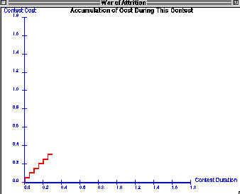
The scales for this plot will be automatically defined according to thecosts and rate at which costs increment. You will see a red line increasein a stepwise manner. Notice that at time zero the cost immediately incrementsby the value you specified in the setup window. This is like the analogywhere players must pay a dollar "upfront" to play in through thenext interval (see expanded description). Recallalso that not paying they money means you quit -- thus quits only occurat the start of the interval and cannot quit at any other time. As longas both contestants continue to play, you will see the costs increment ina stepwise manner. When one or both contestants quit, the graph stopsmoving and a message is posted telling the cost that had been paid whenthe game ended.

Note: Sometimes the coordinate axes for this graph inexplicably donot appear. However, the actual red line graph and summary will still appear;I'm working on this one! As usual I recommend using the latest version ofNetscape or Explorer and there will be fewer problems.

About 2.5 seconds later, this screen will disappear and a summary screenlike the one below will appear:

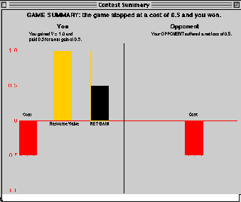
The example above is for a case where one strategy ("you" inthis case) has won. When there is a winner (as above) the screenis divided into results for each of the two competitors. The cost, resourcevalue and net gain are summarized for the winner and the costs alone aregiven for the loser. The there is also text to this effect.

If the contest ends as tie, a more complicated window appearsthat explains how costs and benefits are calculated when ties occur. A smallgreen dialog box that must be resized to be read accompanies this display,it gives details as to the calculations:

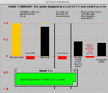
Single GameSimulations --
Things to Try and/or to Think About
What can you do with this simulation? The main use of this simulationis to increase your understanding of the characteristics (behavior) of fixedand mixed strategies in the war of attrition. There is also a secondaryuse -- this module can help increase your understanding of the advantagesand disadvantages of discrete calculations.
Things to try
Cost intervals and precision: It is important to go through thesefirst to get a feel for the limitations of the simulation and the situationswhere you might be misled by what the simulator tells you.

Break the rule about using maximum costs for a fix(x) strategist that is a multiple of delta x. For example, make both contestants identical fix(x=0.29) strategists and set delta x to a couple of values greater than 0.01. Then try 0.01. In other words, try this with costs that are evenly divisible by the cost increment (e.g., 0.40 is evenly divisible by all delta X values) and values that are not (e.g., 0.39 is only even divisible by x = 0 .01). Discussion
Now try the contest with delta x = 0.05 and one contestant at fix(x=0.45) and the other at fix(x=0.5). What do your results tell you about how the contest works (i.e, when are decisions to quit made -- at the start or end of an interval?) What do your results tell you about the relationship between the simulator's cost interval and its ability to determine accurately when a contest has actually ended? Do ties ever occur when you would predict that one or the other should win? Explain. Discussion
Try some cases where a tie should result. Try values of maximum acceptable cost that are evenly divisible by delta x and some that are not. Compare these results with what you saw earlier.
Lastly try some contests when both individuals are 'var' strategists. Does lowering the value of delta x increase you confidence as to how well you knew when the contest ended? Discussion
Let's imagine a real behavioral experiment observing some hypothetical war of attrition between two animals. Suppose that the experimenter only observes the contest at intervals (for example, she is also observing other animals or her view is often blocked). Alternately she observed them continuously but she is using a digital clock. Will she know exactly when quits occurred? Is it possible that she might score a contest as tie (assume she couldn't see the resource) when one or the other animal won? Is there much difference between her situation and this game? Discussion
Once you understand the limits on the accuracy of the simulator's abilityto determine when a contest ends and who won, go on.
Learning About the Fix(x) and 'Var' Strategies
Understanding the Calculation of Benefits and Costs:

Pit two fix(x) strategists against each other and see if the benefits and costs go along with what you would expect. Alter V and be sure you can predict the resulting benefits and costs.
Next, set one of the strategists to be a var strategist. Adopt a large value of x for the remaining fix(x) strategist -- a value between 2 and 5 is good if V >= 1.0 . Repeatedly run the simulation against the same fix(x) opponent and see if the contests seem to be ending as expected.
Do the same as above except change V.
Questions:
1. Does the model behave properly? Did you see examples where ties occurredwhen they should not have happened? If so, do you understand why the machinedeclared a tie and can you pick out cases when it shouldn't have done so?
2. With regards to fix(x) strategists, do the calculations of cost andbenefit make sense to you?
3. With regards to 'var' strategists. When are quits most likely? Doeschanging V in a contest against a given fix(x) strategist do what you mightexpect to quitting times? Discussion
You should gain some appreciation for the predictable unpredictabilityof 'var'. Even though a totally known function underlies its behavior,you can never know when it will quit (short of knowing when its opponentquits).
Unknown Strategist Option:
Once you think that you have gained a good understanding of fix(x) andvar and that you understand how the model works and its limitations, trysetting your opponent as an "unknown" strategist. It will beeasiest to figure out what your opponent is doing if (i) you adopt a relativelyhigh cost fix(x) strategy and (ii) you play the game many times. Playa number of times against different opponents -- there is probably nothingelse that you can do to gain an intuitive understanding of fix and mixed('var') strategies.
Note that if you are a "real animal" you might be playinga 'var' or low max cost strategy -- see if it is as easy to figure outyour opponent's strategy in a given number of contests if you are 'var'or fix(low value x). Think about this; you'll have a better chance to investigatethis in more detail in the multigame section but by all means try it herealso.

Back to the contents and top of this frame
On to the simulation

MultipleGame Simulations

Description: This module differs from the single game simulationin that two given strategists repeatedly play each other a specified numberof times. The computer keeps track of who wins and the payoffs to each player.After the specified number of contests, an output screen displays a frequencydistribution of quitting costs between zero and a user specified maximum.Also, another window appears that gives a text read out of wins by eachcontestant, ties, payoffs and where appropriate, theoretically expectedpayoffs.

Setup: Setup is identical to that for a single game with respectto strategy choice and resourcevalue. The difference is that you will use choice menus to specify

the number of times the contest will be played and
the maximum cost to be plotted on the frequency distribution.

Here is picture of the controls for setting these parameters. Defaultvalues are shown and they are located on the lower part of the MultigameSetup Screen (press here to view the almost identicalsingle game setup screen):

Changing the number of games played will be useful when one orboth contestants are var strategists; it will help to drive home the notionthat var is only predictable within the context of a large number of games.And, as usual, the control can be used to speed up the simulation -- selectinglarge numbers of contests may cause the simulation to take a very long timeon older computers.

The "Output Plot's Max. Cost" choice is useful purelyto allow you to control the resolution of the output screen. Using verylarge values of max. x will tend to obscure results in contests that tendto end at low costs and vice versa. If you select the wrong maximum cost,you can always run the simulation again at a different value. One note:using a low deltaX (0.01 -- high resolution) will prevent you from usingthe largest two maximum costs (5 and 10 *V). This is because the extra resolutioncannot be displayed at these settings on most computer screens (and so nothingis gained). Select a lower maximumx or a larger deltaX.

About the Output Screens: The picture below shows the frequencyof all quits between costs 0 and 1.0 for 5000 repeats of a contest betweena mixed 'var' strategist vs. a fix(x=1.0). Notice that the x axis is cost,and Y axis gives the proportion of individuals quitting after x=0.

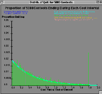
Important note: remember that this is a frequency distribution ofall quits -- by both contestants. The data were deliberately not plottedto show the quits by either types of strategist so that you could use thisplot to try to figure out strategies from quitting patterns.

Thus, it is like the lower graph produced by the Q(x)calculator output except that here there is a single histogram givingthe frequency of quitting at all costs up to the maximum screen x.

Notice also that since one of the strategists is a 'var' strategist,a theoretical plot of frequency of quits (like that given at the bottom of the Q(x) Calculator output) is also plotted forcomparison with the actual proportion of quits. In the case shown, thereis excellent agreement up to the point where fix(x=1.00) quits (and so everyoneelse quits along with it).

Finally, notice that the top of the screen are a number of lines of textthat give the strategies being played, act as legend for the graph and tellwhen the greatest proportion of individuals quit:

Accompanying this plot is yellow textbox that contains additional informationincluding both strategies used, the overall number of wins to each contestant,average payoffs and in the case of 'var' vs. a fix(x), the expected payoffto a 'var'.

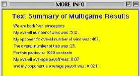
Please note that this window sometimes comes up half empty -- if it does,simply resize it. Also, you will need to move it in order to read all thematerial on the graph. One downside -- if you selected "unknown"this window will tell you the strategy the computer picked. So, don't lookat it until after you have figured out the strategy of your "unknown"opponent.

Multi GameSimulations --
Things to Try and/or to Think About
Things to try
Comparisons Between Observed Data and Theoretical Predictions
Setup 1: Set delta x to 0.01, V to 1, and selecttwo different values for fix(x). Run the simulation and be sure thatit works the way you expect. This will familiarize you with it for the nextsections.
Setup 2:

Set delta x to 0.01, V to 1.0, make one strategist fix(x=1.9) and the other 'var'. This will allow you to run contests that will usually end by 'var' retiring before fix(x) quits (since if V = 1.0, var quits at the rate of about 0.63 per unit x). Select a maximum display x of 2.0.
Run the contest with the settings above at all possible number of repeats (using the "No. Games Played" choice menu). Especially with the low number of games choices, run the game several times at each setting.
Questions on Example#2:

What is the relationship between number of contests run and the degree of fit between the data for cost values less than 1.9 and the theoretical curve?
At cost >= 1.9, are all the quits done by var, fix(x) or both? Explain.
Who won all of the contests at costs < 1.9 or can you say? Explain.
When did ties occur? Explain.
Who won all the contests at cost > 1.9 or can you say? Explain. Discussion of all previous questions
What is the relationship between the actual payoff E(var,fix(x)) (from the simulation results) and the expected (theoretical) payoff as a function of the number of contests?
What is the relationship between the actual payoff E(var,fix(x)) (from the simulation results) and the expected (theoretical) payoff as a function of delta x? Why is the actual payoff usually less than the predicted value? Discussion of the two previous questions
Based on what you know about the symmetrical war of attrition, should E(fix(x=1.9), fix(x=1.9)) be greater than, less than, or equal to E(var, fix(x=1.9))? Explain. Does it bother you that fix(x=1.9) wins most of the contests against var when V=1 -- i.e. that E(fix(x=1.9), var) > E(var, fix(x=1.9))? After all, var is supposed to be an ESS. Discussion
Setup 3: Make both contestants 'var'. Run the simulation usingdifferent numbers of contests. Remember that the histogram output is totalquits (both contestants added together) and the theoretical line is forexpected quits for a single contestant playing var.
Questions on Example#3:
Is there good agreement between the theoretical line and the actual data?If not, explain what you think is the cause of the difference and attemptto explain any differences you might observe. Discussion
Setup 4: Set your opponent to "unknown" and select astrategy for yourself. Try to determine the unknown strategy without readingthe yellow box. What is the relationship between strategy used and numberof contests and your accuracy of determining the opponent's strategy?

Back to the contents and top of this frame
On to the simulation

Value of V	Proportion Quitting for a Given V
0.3	0.154
1.0	0.049
3.0	0.017

Value of V	Proportion Quitting for a Given V	Normalized Proportion Quitting for a Given V
0.3	0.154	1.0
1.0	0.049	0.32
3.0	0.017	0.11