Graphs of Net Benefits, Costs, and Payoffs for Fix(x) and
'Var'
Graphs For Fix(x=m):
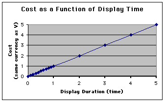
The first curve is very simple -- it just shows that we assume that costs
increase linearly (with a slope of 1) over time.

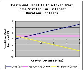
This next graph once again shows the costs that are paid (blue line,
same as above) and adds resource value (violet) and net benefit (V-m). Resource
value is, of course, constant and independent of cost. Therefore in longer
contests with greater costs, the net resource value (i.e. the net gain from
winning) eventually becomes negative:

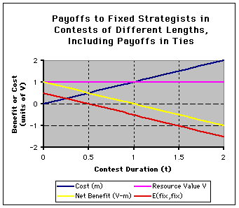
The final graph (below) compares costs, resource value, net benefit,
and payoffs in ties. As before, costs are a linear slope = 1 function of
time, resource value is constant and net benefit is (V-m).
Now:
- the payoff to fix(x) in a given length contest if it wins is the net
benefit curve which equals (V-m).
- If fix(x) loses, it costs fix(x) m and it gains nothing.
- In the ties that we are interested in, the payoff E(fix(x=m),
fix(x=m)) must be the sum of half of each of these quantities since we
assume that fix(x) divides the resource in ties.
- Thus, fix(x=m) gets the resource 0.5 of the times and so when it does
it gains 0.5(V-m).
- It also doesn't get the resource 0.5 of the times and loses 0.5 *m.
Thus, overall, E(fix(x=m), fix(x=m)) is the sum of these: 0.5(V-m) -
0.5m = 0.5V-m.
This is graphed as the red line below:

For the Mixed Strategy 'Var':

Before Continuing, Let's Be Certain
That
We Understand This Graph.
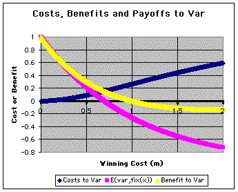
Axes:
- The Y axis is either cost, benefit or payoff; all are
in the same units as V. As usual we show costs as positive values (our
convention then is to subtract costs from benefits. By the same token,
net benefit in winning (yellow line) can be positive (if V > cost of
winning V), negative (if V < cost of winning V) or neither.
- The X axis is the cost x.
It is extremely important that you realize that all of the curves
above are lifetime or theoretical curves. Thus,
the payoff curve (magenta) is the solution giving the lifetime payoff
to a var strategist when pitted against a all possible cost fix(x)
strategist if V=1.0.
Thus, the particular fixed strategist that var is playing
is given as the x axis value. For example: E(var, fix(0.5V))
= 0.212V; E(var, fix(0.2 V)) = 0.64V, etc. |
Now, let's see what is interesting about this graph:
- Net Benefits when 'var' wins vary between V and values less
than zero but greater than -V. At high values of m net Benefits again approach
zero. The only part of this that is difficult to understand is why
net benefits do not continue to decrease as contests get longer.The reason
is that it is very rare for 'var' to display to a high cost relative
to the value of the resource.
Recall that 'var' tends to quit most contests at relatively low costs
(press here to review
the plot of the chance that 'var' will play to some given cost (given
its opponent has not quit)).
- Since high cost contests are very rare for 'var', then the "lifetime
benefit" in these contests is very low -- over a lifetime 'var' receives
the net benefit commensurate with a given cost contest times the proportion
of times it plays to this cost -- essentially zero.
- COSTS in losses are also constrained, this time between 0
and +V (see a graph).
- Recall from equation 16a that when calculating the lifetime cost of losses
to a given fix(x) strategist one had to sum the products of the probability
of each of those losses and their cost.
- Now, imagine an opponent who plays fix(x = high cost).
- Low cost losses to this opponent are common (since 'var' quits at low
costs most frequently (review)); high cost losses become increasingly less likely
as the cost increases and so the total lifetime cost tends to increase
very little as fix(x) opponents of larger cost are compared to those of
intermediate costs.
- PAYOFFS: The result is that E(var,fix(x)) varies between V and -V.
By contrast, E(fix(x), fix(x)) varies between +V and (potentially) negative
infinity (see eq. 19). Again, the reasons should be obvious --
- in contests with an m of just slightly more than zero there
is essentially no cost and so the winner gains essentially V.
- in a contest that lasts infinitely long, the lifetime benefits of such
a contest are near zero. However, these contests are infinitely rare and
therefore the net benefit of long contests is essentially zero.
- by contrast, costs are always paid in any contest, whether the focal
individual wins or loses.
- Thus, even though it is very unlikely that a var strategist
will play extremely long, to the extent that they do they play a very large
cost. And since the rate of quitting is a function of V (rate = 1/V), as
the cost gets greater the chance of paying the cost becomes less and the
product of the two converge at V.
- E(var,fix(x)) is positive at any opponent's quitting cost that is
less than 0.693*V. By contrast, E(fix(x),fix(x)) is positive only at
costs less than 0.5V.
