Part 1: What is an exponential decay -- an example: As mentioned in the main text, exponential decay occurs when a constant probability per unit of independent variable acts on all members of a population. Suppose that time is our independent variable and metric of cost (as in the war of attrition). There is a certain chance of continuing per unit of time. Likewise, there is also a certain chance of quitting per unit cost that equals 1 - chance of continuing. These chances act on all members of the study population. If we now look at the number of individuals in the game at any time, we will see that the result of this constant probabilities acting on all individuals is that that the number of individuals still in the game will decrease rapidly at first and then more slowly as it approaches zero.
Here is an example that illustrates exponential decays and should make clear why a constant probability can result in different absolute numbers of individuals quitting in different intervals. To make this easy to understand, let's make time a discrete variable. We'll assume that it increments in 5 s. amounts. There is a certain chance of continuing from one of these 5 s. intervals to the next. Let's say it is 90% (in other words, there is a 0.1 chance of quitting each 5 s.). Let's also say that decisions as to whether or not to quit or continue occur at exactly 5 s. intervals.
Now imagine a starting population of 1000 individuals. Alternately, imagine a single individual who will play the game 1000 times (like the lifetime of a 'var' strategist). At time zero we have 1000 contestants (or the single individual starts the contest 1000 times). At 5 s.we reach the first decision point. There is 0.9 chance that each individual will continue (i.e., there is a 0.9 chance that our single individual will continue in a given contest). So after the 5 s. decision, 90% of the individuals continue -- i.e., 900 remain. Ten percent quit the game (100 individuals) and so they are no longer members of the population (alternately, our single player is still in the game 900 out of the 1000 times he plays). At 10 s. there is another decision point. Once again there is a 90% chance of continuing acting on each player. After this decision, there are 810 individuals left -- this time 90 quit (alternately, our single player is still playing 810 times out of 1000 starts and there were 90 quits at time = 10 s. And so on.
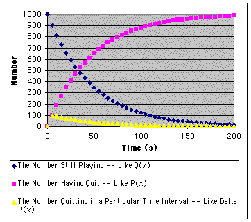
Here are graphs of the results of this game:

Follow the blue dots. This is the population size (or number of times a single individual) is still playing after paying a given cost. Put another way, for a given time cost, the blue plot is the number of individuals out of 1000 who will be expected to pay that cost (or the number of times a single individual will be expected to pay that particular time cost. Thus, the blue plot is closely related to the cumulative probability of continuing plot, Q(x). Notice that this plot decreases most rapidly at first (as shown by the largest number of quits occuring at t = 5 s -- see the yellow plot. At each subsequent time cost, the blue plot becomes less steep as the population gradually approaches zero.
About the Other Plots in the Graph Above It's a good time to look to look at the other two plots. The violet symbols show the number of individuals who have quit as of any cost x. It is simply the difference between the number that started and the number who are still playing. It is essentially the same as a plot of the equation for P(m) The plot with yellow symbols shows the number that quit in a specific interval. Thus, it is the same as the "delta P(m)" function that we studied earlier. Notice that after time zero (when no one quit in this game) it also follows an exponential decay. |
Thus, an exponential decay is characterized by a slowing of the absolute decrease of the dependent variable (here number of times or individuals) as the independent variable (time in this example) increments. It is the result of a constant chance acting on the remaining population -- in our example each individual has a constant 90% chance of remaining each 5 s.
Part 2: The equation for exponential decay: Now, we can write a generalized equation for the blue plot (above) as:
where Y is the dependent variable (e.g., number still playing or number of times still playing), k is a constant (in the example we are considering it is 1000, the total number of contestants or number of times an individual plays the game), e or exp() is the base of the system of natural logarithms, approximately 2.718, x is the present cost (in our example, it will be either zero of multiples of 5 but in other cases, it could have any value) and r is the rate constant which determines how rapidly the dependent variable (Y or number in our example) decreases per unit cost.
Let's look into the rate constant a bit more. First, notice that the expression e^(-r) gives the actual rate of decrease per unit x. Now, since we know that for our example, there is a 0.9 chance of remaining per 5 s., then:
exp(-r) = 0.9
taking the antilog of this equation gives us the value of r
r = 0.1054 individuals or contests / 5s = 0.021 individuals or contests / s
Which of these values we use for r will depend on how we enumerate cost -- if we give it as seconds since the start of the contest (and calculate only at values of 0, 5, 10, 15 etc. s.) then we use 0.021, if we count intervals such that x = 5 s. then we use r = 0.1054 and use values of x of 0 , 1 (for 5 s.), 2 (for 10 s.) etc.
Finally, notice that the multiplying the rate constant by the independent variable (cost) gives us a change appropriate to all sorts of x intervals.
Try the following problems, all based on the example above:
Problems Dealing With Rate Constants and The Exponential Decay Equation (try these to be sure you understand the material above) Assume that cost is enumerated in 5 s. intervals i.e., decisions are made every 5 s. Therefore, if the chance of continuing each 5 s. is 90%, then r = 0.1054. If an individual plays the contest 1000 times: 1a. How often will he still be playing at x = 5 s? x= 10 s? Answer 1b. How often will he play till 35 s.? Answer Now assume that individuals can decide each second whether or not to continue. Once again, the chance of continuing over 5 s. is 90% and so r = 0.02107 2. How often will he still be playing at x = 5 s? x= 10 s? Answer Assume that individuals can decide each second whether or not to continue (as in the last problem). The chance of continuing over 5 s. is 90% 3a. What is the chance of quitting each 5 s.? Answer 3b. What is the chance of quitting each second? (Hint: the chance of quitting each second must add to the total chance over 5 s.). Answer 3c. What is the chance of continuing each second? (Hint: remember that total probability for any unit x must add to 1.0. Use this fact and your answer to 3b to answer this question). Answer 3d. Take your result for the chance of continuing per second (#3c) and find r per second. Compare this value with the one given in question #2 (r = 0.02107). Answer 3e. Take your answer in 3c and multiply it together 5 times. What do you get? Answer |
Part 3: Equation #6 (probability density function) as Exponential Decay: It should now be easy to see why equation 6:
eq. #6:  |
is an equation of exponential decay.
The only slightly confusing aspect is the rate constant. In eq. 6, r = 1/V.
Just like in the
generalized equation above, the larger the rate constant, the faster the
decay of the dependent variable. Thus, in this case, the faster the
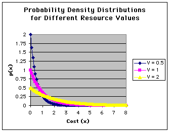
probability per unit cost decreases. This is evident if we look at plots
of eq. 6:

Now since the rate constant is 1/V in the case of eq. 6, then as V increases, the rate constant decreases. This is evident in the shallower slopes with higher rate constants.
The larger the value of the resource V compared to a unit of cost x, the greater the cost an animal should be willing to pay when displaying for that resource. The reason should be obvious -- net benefit is what matters and if the resource is more valuable, it a greater cost can be borne before the resource costs more than it is worth!
One thing might puzzle you however. Why should plots of p(x) start at higher probability densities as V decreases? The reason is that we would expect most quitting to occur at low costs if V is also low. So, the density of probability values (the chance of quitting per unit x) would be greatest at these low values of x. That is why k in eq.# ed1 is 1/V.
This is a good time to review the idea of probability density or see how k was found for eq. 6.